Bias in stratum-specific abundance estimates

Author

Centre for Research into Ecological and Environmental Modelling
University of St Andrews

Published

March 22, 2024

Demonstration

Distance sampling simulation where detection functions differ between strata. When stratum-specific abundance estimates are produced using a pooled detection function, bias arises. The magnitude of the bias depends upon the magnitude of the difference in the detection functions.

Introduction

We tell participants in the introductory distance sampling workshop of the perils of estimating stratum-specific densities when using a pooled detection function (Buckland et al., 2015, Sect. 2.3.1). Therefore, if the purpose of the study is to produce stratum-specific density estimates, sufficient effort must be allocated per stratum to support stratum-specific detection functions. It might be the case that multiple strata share the same detection function, but reliance upon luck for that to occur is not the basis for sound inference. Sufficient detections should be made in each stratum to assess whether strata share a common detection function.

This simulation study evaluates the magnitude of bias in stratum-specific density estimates when strata differ in the scale parameter of their detection functions.

library(dsims)

Loading required package: dssd

library(leaflet)
library(knitr)
library(sf)

Linking to GEOS 3.11.2, GDAL 3.7.2, PROJ 9.3.0; sf_use_s2() is TRUE

library(here)

here() starts at C:/Users/erexs/Documents/GitHub/Oct-Quarto

Study area

The only interesting feature of the study area used in this simulation is that it possesses two strata. We could have employed more strata, but demonstration of the phenomenon is sufficient with only two strata.

myshapefilelocation <- here("shapefiles", "StrataPrj.shp")
northsea <- make.region(region.name = "minkes",
                      shape = myshapefilelocation,
                      strata.name = c("South", "North"),
                      units = "km")

North Sea study area

Interest is in estimating the density of minke whales in the western portion of the North Sea, off the east coast of Britain. The study area is divided into north and south strata, with the north stratum being roughly 1.9 times the size of the south stratum, as shown in the map below.

m <- leaflet() %>% addProviderTiles(providers$Esri.OceanBasemap)
m <- m %>% 
  setView(1.4, 55.5, zoom=5)
minkes <- read_sf(myshapefilelocation)
study.area.trans <- st_transform(minkes, '+proj=longlat +datum=WGS84')
m <- addPolygons(m, data=study.area.trans$geometry, weight=2)
m

Population specification

Population is evenly distributed (density surface is horizontal) and the population size is apportioned to the strata according to the stratum size. This should result in both strata having the same density.

areas <- northsea@area
prop.south <- areas[1]/sum(areas)
prop.north <- areas[2]/sum(areas)
total.abundance <- 3000
abund.south <- round(total.abundance * prop.south)
abund.north <- round(total.abundance * prop.north)
constant <- make.density(region = northsea, x.space = 10, constant = 1)
minkepop <- make.population.description(region = northsea,
                                           density = constant,
                                           N = c(abund.south, abund.north))

Survey design

Specifying a single value for the number of samples will distribute the transects among strata proportional to the stratum sizes. Emphasis of this simulation study is not upon the properties of the survey design, therefore a simple systematic parallel line transect survey is created. Note however, there is large number of replicate transects in each stratum; a well-designed study. Any bias in the estimated densities cannot be attributed to poor design.

coverage.grid <- make.coverage(northsea, n.grid.points = 100)
equal.cover <- make.design(region = northsea,
                           transect.type = "line",
                           design = "systematic",
                           samplers=40, 
                           design.angle = c(50, 40),
                           truncation = 0.8,
                           coverage.grid = coverage.grid)

Properties of the design

To demonstrate the estimated number of transects in each stratum, the run.coverage function is used to show the number of replicates in each stratum is allocated roughly according to stratum size.

design.properties <- run.coverage(equal.cover, reps = 10, quiet=TRUE)
mine <- data.frame(Num.transects=design.properties@design.statistics$sampler.count[3,],
                   Proportion.covered=design.properties@design.statistics$p.cov.area[3,])
kable(mine)

	Num.transects	Proportion.covered
South	17	8.10
North	23	8.11
Total	40	8.12

What analysis to conduct

For purposes of this investigation, we look only at the same key function under which the data were simulated (the half normal) with no covariates. In effect we are using the “wrong model” to make inference, except in the circumstance when \(\Delta = 1\).

A second analysis, strat.specific.or.not is constructed to assess model selection performance: the “wrong” model is paired with the “correct” model that assumes stratum-specific detectability. This contrast will measure the ability of AIC to choose the correct model as the difference between stratum-specific scale parameters (\(\Delta\)) changes.

pooled.hn <- make.ds.analysis(dfmodel = list(~1),
                                key = "hn",
                                criteria = "AIC",
                                truncation = 0.8)
strat.specific.or.not <- make.ds.analysis(dfmodel = list(~1, ~Region.Label),
                                key = "hn",
                                criteria = "AIC",
                                truncation = 0.8)

Heart of the simulation

Loop over \(\Delta\) difference in \(\sigma\) between strata

delta.multiplier <- c(seq(from=0.5, to=1.1, by=0.1),
#                      seq(from=0.85, to=1.15, by=0.1),
                      seq(from=1.2, to=2.4, by=0.2))
sigma.south <- 0.3
north.sigma <- sigma.south*delta.multiplier

Scale parameter (\(\sigma\)) for the southern stratum remains fixed at 0.3, but in the northern stratum, the scale parameter is a multiple of the southern stratum \(\sigma\), ranging from a low of 0.15 to a maximum of 0.72.

hn <- function(sigma, x) {return(exp(-x^2/(2*sigma^2)))}
for (i in seq_along(north.sigma)) {
  curve(hn(north.sigma[i],x),from=0,to=0.8,add=i!=1,  
        xlab="Distance", ylab="Detection probability", 
        main="Range of detection probability disparity\nSouth function in blue")
}
curve(hn(sigma.south,x),from=0,to=0.8, lwd=2, col='blue', add=TRUE)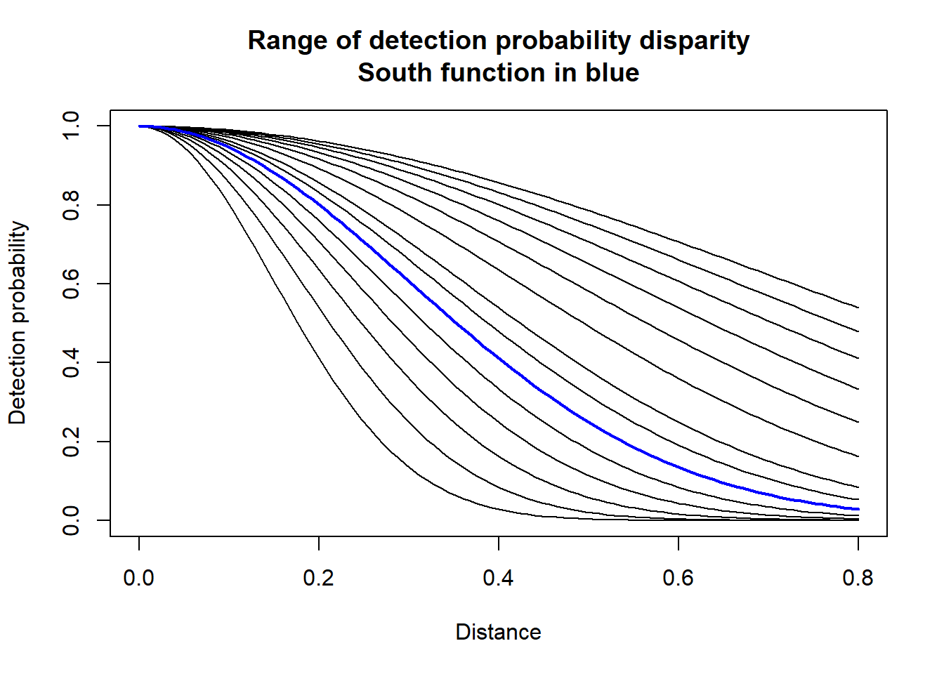

equalcover <- list()
whichmodel <- list()
num.sims <- 10
for (i in seq_along(delta.multiplier)) {
  sigma.strata <- c(sigma.south, sigma.south*delta.multiplier[i])
  detect <- make.detectability(key.function = "hn",
                               scale.param = sigma.strata,
                               truncation = 0.8)
  equalcover.sim <- make.simulation(reps = num.sims,
                                    design = equal.cover,
                                    population.description = minkepop,
                                    detectability = detect,
                                    ds.analysis = pooled.hn)
  whichmodel.sim <- make.simulation(reps = num.sims,
                                    design = equal.cover,
                                    population.description = minkepop,
                                    detectability = detect,
                                    ds.analysis = strat.specific.or.not)
  equalcover[[i]] <- run.simulation(equalcover.sim, run.parallel = TRUE, max.cores=7)
  whichmodel[[i]] <- run.simulation(whichmodel.sim, run.parallel = TRUE, max.cores=7)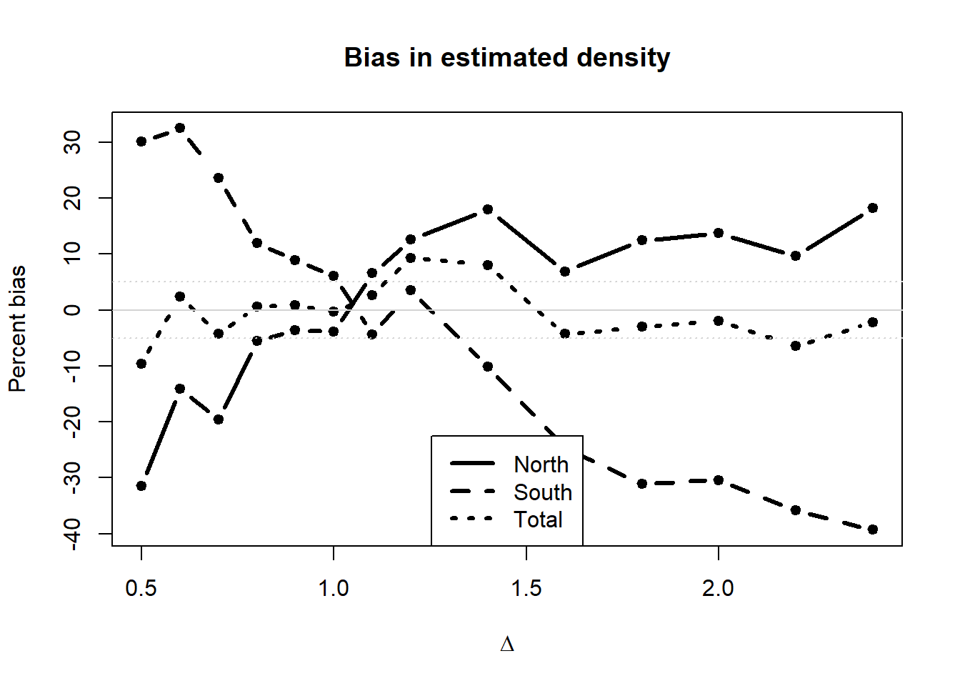
}

Simulation findings

Tabular results of simulations iterating over the range of \(\Delta\) values for the scale parameters of the two strata. As \(\Delta\) approaches 1, the two detection functions converge, hence using the pooled detection function is appropriate. When \(\Delta>1\) bias again increases, however because for values of \(\Delta>>1\), the detection function for the North stratum becomes nearly horizontal. The number of detections in the North stratum is becoming asymptotic. There is little margin for bias to arise in the North density estimate; bulk of bias arises from estimates in the South stratum.

The final column of the table indicates the proportion of replicates for which the stratum-specific detection function is selected using AIC. The stratum-specific detection function model is the “correct” model when \(\Delta \neq 1\). However the stratum-specific detection function model is selected \(\approx\) 20% of the time when \(\Delta \approx 1\). More troubling, the stratum-specific detection function model is selected <50% of the time when \(\Delta \neq 1\) implying the “incorrect” model using a pooled detection function is selected >50% of the time, even for large values of \(\Delta\).

Results using pooled detection function
	Bias.N	Bias.S	Bias.Tot	CICover.N	CICover.S	CICover.Tot	Detects.N	Detects.S	Detects.Tot	Prop.strat.model
0.5	-31.5	30.0	-9.7	0.3	0.7	0.9	38	40	78	1.0
0.6	-14.1	32.4	2.4	0.8	0.8	1.0	48	41	89	1.0
0.7	-19.6	23.5	-4.3	0.7	0.8	1.0	50	43	93	1.0
0.8	-5.6	11.9	0.6	0.9	1.0	1.0	60	39	99	0.9
0.9	-3.7	8.9	0.8	1.0	0.9	1.0	68	42	109	0.2
1	-3.9	6.1	-0.3	0.9	1.0	0.9	71	43	114	0.2
1.1	6.5	-4.4	2.7	1.0	0.8	1.0	82	40	122	0.3
1.2	12.5	3.5	9.3	0.8	0.8	0.7	89	45	134	0.2
1.4	18.0	-10.1	8.0	0.7	0.9	0.9	100	42	142	0.8
1.6	6.9	-24.7	-4.3	1.0	0.6	1.0	105	40	146	0.9
1.8	12.4	-31.0	-3.0	0.9	0.4	0.9	114	38	152	0.9
2	13.7	-30.4	-1.9	0.5	0.6	0.8	125	42	166	0.9
2.2	9.6	-35.8	-6.5	0.9	0.3	0.8	130	42	172	1.0
2.4	18.2	-39.3	-2.2	0.8	0.2	0.9	131	37	168	1.0

When employing model selection to choose between models with pooled detection functions and stratum-specific detection functions, the most worrisome cases of bias arising when \(\Delta << 1\) are eliminated. Bias in stratum-specific density estimates become more pronounced as \(\Delta >> 1\).When \(\Delta\) is at its maximum, the probability of using the model that produces unbiased stratum-specific estimates is 1

Bias in density estimates when using model selected using AIC.
	Bias.N	Bias.S	Bias.Tot	CICover.N	CICover.S	CICover.Tot
0.5	0.1	-5.8	-2.0	1.0	1.0	1.0
0.6	0.3	-3.3	-0.9	1.0	0.9	1.0
0.7	-6.4	0.4	-4.0	1.0	0.9	1.0
0.8	6.3	-8.6	1.0	1.0	1.0	1.0
0.9	-5.3	0.1	-3.4	1.0	0.9	1.0
1	-0.7	-0.1	-0.5	0.9	1.0	1.0
1.1	0.1	-12.4	-4.3	1.0	0.8	1.0
1.2	-0.5	-10.4	-4.0	1.0	0.8	1.0
1.4	-2.3	-1.9	-2.1	0.8	1.0	1.0
1.6	-5.6	-1.7	-4.2	1.0	0.9	1.0
1.8	5.4	9.1	6.7	0.9	0.8	1.0
2	0.1	-7.5	-2.6	1.0	0.9	1.0
2.2	0.1	8.2	3.0	1.0	1.0	0.9
2.4	-1.2	0.1	-0.7	1.0	1.0	0.9

Conclusions from this portion of study

Note bias in the estimated density for the entire study area is never greater than 10%, yet another demonstration of pooling robustness. Even with widely differing detection functions, the estimated density ignoring stratum-specific differences is essentially unbiased.

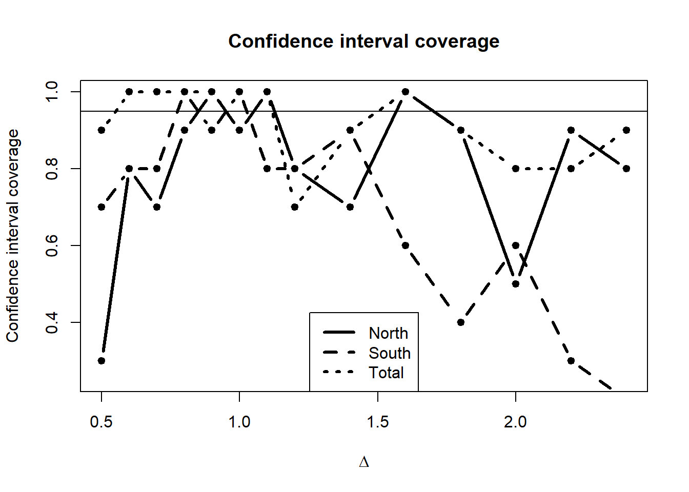
Confidence interval coverage for stratum-specific estimates approaches nominal levels when \(\Delta \approx 1\). Coverage for the density estimate in the entire study area is nominal for all values of \(\Delta\) with the exception of \(\Delta<0.7\).

Model selection sensitivity

This small simulation demonstrates the peril of making stratum-specific estimates when using a detection function that does not recognise stratum-specific detection function differences. This situation can arise when numbers of stratum-specific detections are too small to support stratum-specific detection functions. This set of simulations was devised such that there was sufficient effort in each stratum to avoid small numbers of detections. Even so, use of the “wrong” (pooled) detection function leads to considerable bias in density estimates.

plot(delta.multiplier, modelsel, 
     main="Stratum-specific model chosen", type="b", pch=20,
     xlab=expression(Delta), ylab="Stratum covariate chosen")
abline(h=0.50)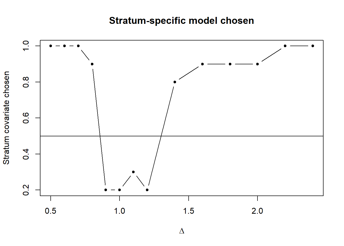

There are two messages from this model selection assessment. Only when \(\Delta < 0.8\) or \(\Delta > 1.2\) is there a better than even chance AIC will detect the difference in detectability between strata. Values of \(\Delta\) in this region do not lead to extreme bias in stratum-specific density estimates when the pooled detection function model is used. There is roughly a 10% negative bias in density estimates of the north stratum and a 5% positive bias in density estimates of the southern stratum.

References

Buckland, S. T., Rexstad, E. A., Marques, T. A., & Oedekoven, C. S. (2015). Distance sampling: Methods and applications. Springer.