library(dssd)
library(sf)
Linking to GEOS 3.13.1, GDAL 3.10.2, PROJ 9.5.1; sf_use_s2() is TRUEDistance sampling survey design
library(dssd)
library(sf)Linking to GEOS 3.13.1, GDAL 3.10.2, PROJ 9.5.1; sf_use_s2() is TRUEWhat spacing would you select for this design? What is the maximum trackline length for the design you have selected? What on-effort line length are we likely to achieve?
The spacing chosen by
dssdof 4937.5m to generate a line length of 200km resulted in a maximum trackline length of around 261km (each exact answer will vary due to the random generate of surveys). If we choose this design then it is possible that when we randomly generate our survey we may not be able to complete it with the effort we have available.
We should therefore increase the spacing between the transects and re-run the coverage simulations. A spacing of 5000m gave a maximum trackline length of around 249km (see summary table of Trackline length in the output below) so we can be fairly confident that we will be able to complete any survey which we randomly generate from this design. This spacing should allow us to achieve an on-effort line length of 199km (see Line length section of design summary below). The minimum line length we would expect to achieve is 184km and the maximum is 206km. [Note your values might differ to those below]
shapefile.name <- system.file("extdata", "StAndrew.shp", package = "dssd")
region.sab <- make.region(region.name = "St Andrews Bay",
                      units = "m",
                      shape = shapefile.name)
cover.sabay <- make.coverage(region.sab, n.grid.points = 5000)
design.spacing5km <- make.design(region = region.sab,
                      transect.type = "line",
                      design = "systematic",
                      spacing = 5000,
                      design.angle = 90,
                      edge.protocol = "minus",
                      truncation = 2000,
                      coverage.grid = cover.sabay)
design.spacing5km <- run.coverage(design.spacing5km, reps = 250, quiet=TRUE)
plot(design.spacing5km)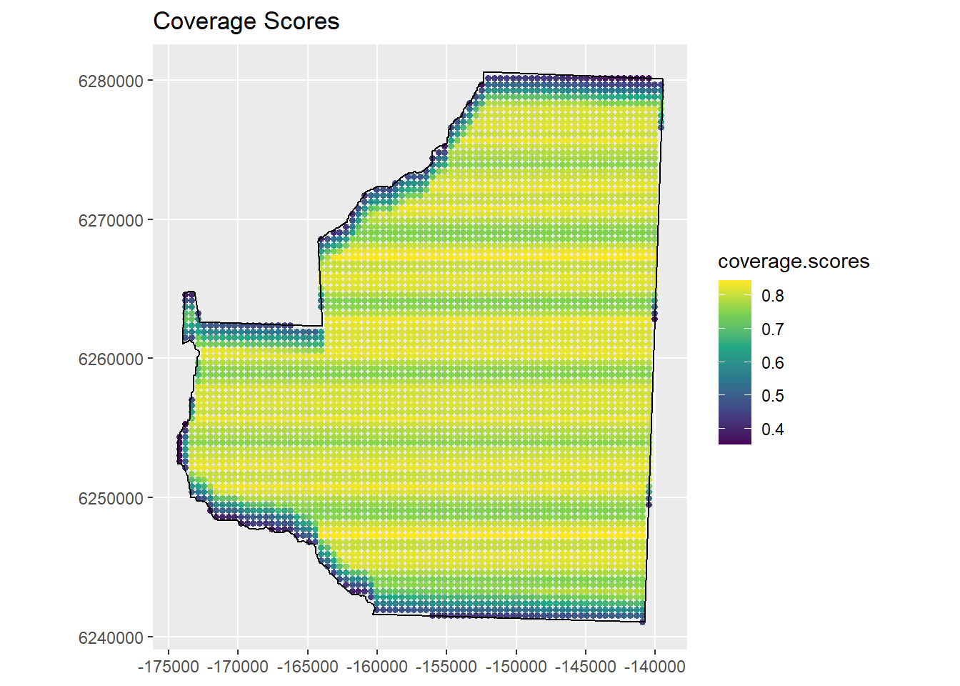
print(design.spacing5km)
   Strata St Andrews Bay:
   _______________________
Design:  systematically spaced transects
Spacing:  5000
Number of samplers:  NA
Line length: NA
Design angle:  90
Edge protocol:  minus

Strata areas:  987500079
Region and effort units:  m
Coverage Simulation repetitions:  250

    Number of samplers:

        St Andrews Bay Total
Minimum            7.0   7.0
Mean               7.9   7.9
Median             8.0   8.0
Maximum            8.0   8.0
sd                 0.3   0.3

    Covered area:

        St Andrews Bay     Total
Minimum      726055570 726055570
Mean         760407417 760407417
Median       766130222 766130222
Maximum      778652197 778652197
sd            15935049  15935049

    % of region covered:

        St Andrews Bay Total
Minimum          73.52 73.52
Mean             77.00 77.00
Median           77.58 77.58
Maximum          78.85 78.85
sd                1.61  1.61

    Line length:

        St Andrews Bay     Total
Minimum      184432.64 184432.64
Mean         197560.90 197560.90
Median       198999.63 198999.63
Maximum      205765.97 205765.97
sd             6198.49   6198.49

    Trackline length:

        St Andrews Bay     Total
Minimum      220528.16 220528.16
Mean         241884.77 241884.77
Median       246210.05 246210.05
Maximum      248800.84 248800.84
sd             8665.07   8665.07

    Cyclic trackline length:

        St Andrews Bay     Total
Minimum      251938.84 251938.84
Mean         278597.75 278597.75
Median       283667.19 283667.19
Maximum      285987.23 285987.23
sd            10197.36  10197.36

    Coverage Score Summary:

        St Andrews Bay      Total
Minimum     0.35200000 0.35200000
Mean        0.76982873 0.76982873
Median      0.80000000 0.80000000
Maximum     0.84400000 0.84400000
sd 0.08780287 0.08780287Does this design meet our survey effort constraint? What is the maximum total trackline length for this design? What line length are we likely to achieve with this design? Is this higher or lower than the systematic parallel design?
You were asked to then run a coverage simulation and check if the trackline length was within our effort constraints. I found the maximum trackline length to be 242km (see Trackline length summary table in the output below) so within our constraint of 250km. I then got a mean line length of 221km and minimum and maximum line lengths of 212km and 227km, respectively (see Line length summary table in the output below). We can therefore expect to achieve just over 20km more on-effort survey line length with the zigzag design than the systematic parallel line design - 10% gain. [Note your values may differ]
design.zz.4500 <- make.design(region = region.sab,
                      transect.type = "line",
                      design = "eszigzag",
                      spacing = 4500,
                      design.angle = 0,
                      edge.protocol = "minus",
                      bounding.shape = "convex.hull",
                      truncation = 2000,
coverage.grid = cover.sabay)design.zz.4500 <- run.coverage(design.zz.4500, reps = 250, quiet=TRUE)
# Plot coverage
plot(design.zz.4500)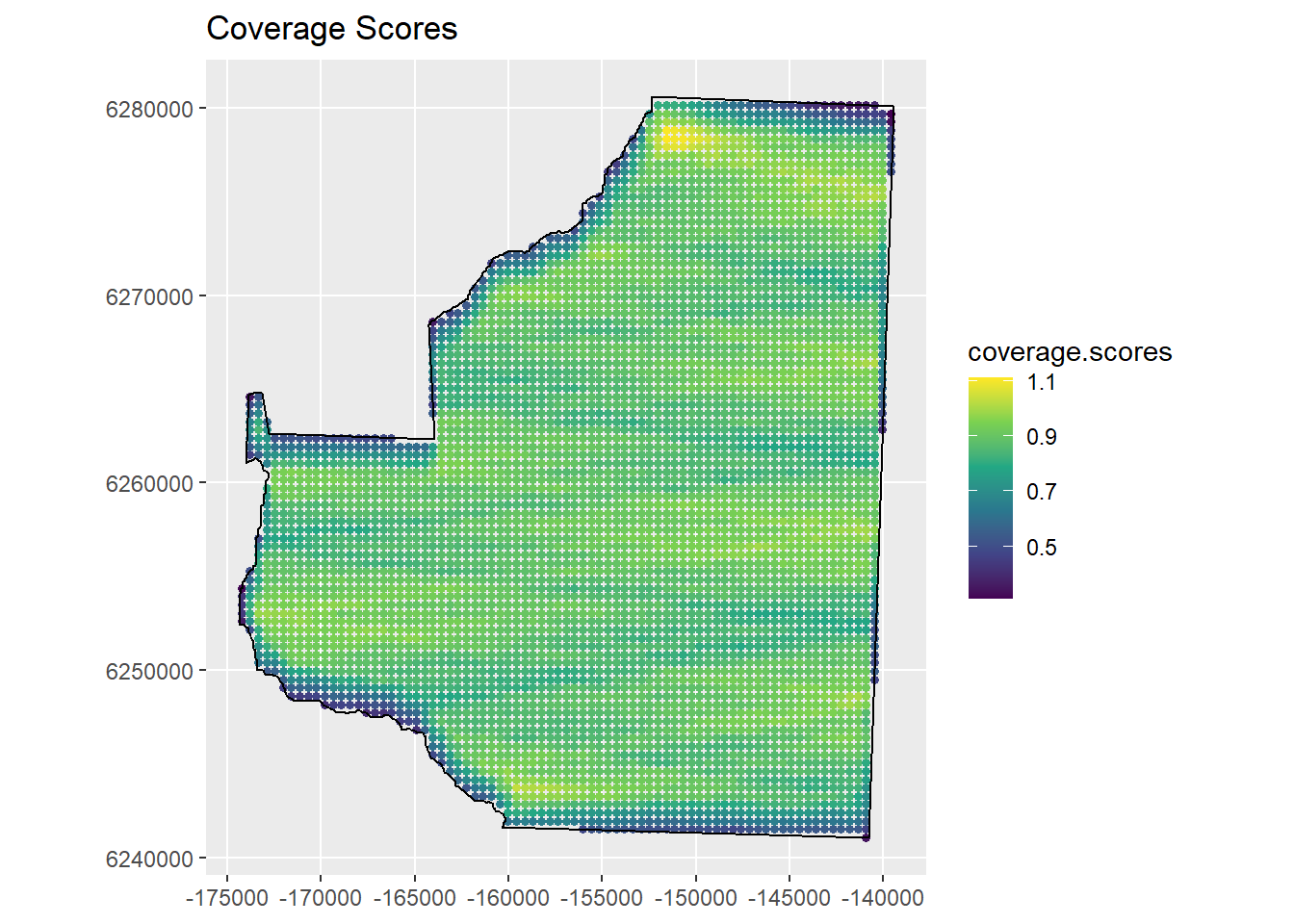
Do you think the coverage scores look uniform across the study region? Where are they higher/lower? Why do you think this is?
You were finally asked to look at the coverage scores across the survey region to see if this design has even coverage. There are some points with lower coverage around the survey region boundary. This is actually down to the fact we are using a minus sampling strategy. If we plotted coverage scores from a systematic parallel design we would see a similar pattern. Usually edge effects from minus sampling are minor unless we have a very long survey region boundary containing a small study area. If the fact that we are using a zigzag design was causing us issues with coverage we would expect to see higher coverage at the very top or very bottom of the survey region (as our design angle is 0). We do not see this. The survey region boundaries at the top and bottom are both quite wide and perpendicular to the design angle, in this situation zigzag designs perform well with regard to even coverage.
What are the analysis implications of a design with unequal coverage?
As our two strata have different coverage we should analyse them separately. We therefore need to make sure that we have sufficient transects in each strata to perform an analysis - ideally 20. There are two reasons that we should analyse them separately. Firstly, our covered area will not be representative of the study area as a whole. If density is higher or lower in one strata than the other we will get a biased estimate of abundance for the area as a whole using the standard distance sampling estimators. Secondly, pooling robustness between the two strata will no longer apply and it may be the case that detection functions differ between the two strata. We will no longer have a representative sample of observations across the entire study region either.
Organise the study area shape file.
shapefile.name <- system.file("extdata", "TentsmuirUnproj.shp",
                              package = "dssd")
sf.shape <- read_sf(shapefile.name)
st_crs(sf.shape)
Coordinate Reference System:
User input: WGS 84
wkt:
GEOGCRS["WGS 84",
DATUM["World Geodetic System 1984",
ELLIPSOID["WGS 84",6378137,298.257223563,
LENGTHUNIT["metre",1]]],
PRIMEM["Greenwich",0,
ANGLEUNIT["degree",0.0174532925199433]],
CS[ellipsoidal,2],
AXIS["latitude",north,
ORDER[1],
ANGLEUNIT["degree",0.0174532925199433]],
AXIS["longitude",east,
ORDER[2],
ANGLEUNIT["degree",0.0174532925199433]],
ID["EPSG",4326]]proj4string <- "+proj=aea +lat_1=56 +lat_2=62 +lat_0=50 +lon_0=-3 +x_0=0
+y_0=0 +ellps=intl +units=m"
projected.shape <- st_transform(sf.shape, crs = proj4string)
region.tm <- make.region(region.name = "Tentsmuir",
strata.name = c("Main Area", "Morton Lochs"),
shape = projected.shape)Create the coverage grid.
cover.tm <- make.coverage(region.tm, n.grid.points = 5000)
design.tm <- make.design(region = region.tm,
                         transect.type = "point",
                         design = "systematic",
                         samplers = c(25,15),
                         design.angle = 0,
                         edge.protocol = "minus",
                         truncation = 100,
                         coverage.grid = cover.tm)
survey.tentsmuir <- generate.transects(design.tm)print(survey.tentsmuir)
   Strata Main Area:
   __________________
Design:  systematically spaced transects
Spacing:  751.2295
Number of samplers:  26
Design angle:  0
Edge protocol:  minus
Covered area:  792161.6
Strata coverage: 5.61%
Strata area:  14108643

   Strata Morton Lochs:
   _____________________
Design:  systematically spaced transects
Spacing:  218.3674
Number of samplers:  14
Design angle:  0
Edge protocol:  minus
Covered area:  389312.9
Strata coverage: 54.43%
Strata area:  715264.9

   Study Area Totals:
   _________________
Number of samplers:  40
Covered area:  1181475
Average coverage: 7.97%What spacing was used in each strata to try and achieve the desired number of samplers? Did your survey achieve exactly the number of samplers you requested? How much does coverage differ between the two strata for this realisation?
A spacing of 751m was used in the main stratum and 218m in the Morton Lochs stratum - these values are calculated based on the stratum areas and should not vary between surveys generated from the same design. You may or may not have achieved the number of transects you requested, this will depend on the random start point calculated for your particular survey. There will also be some variability in coverage, my survey achieved a coverage of 5.7% in the main strata and 64.8% in the Morton Loch strata.
coverage.tentsmuir <- run.coverage(design.tm, reps=250, quiet=TRUE)
print(coverage.tentsmuir)
   Strata Main Area:
   __________________
Design:  systematically spaced transects
Spacing:  NA
Number of samplers:  25
Design angle:  0
Edge protocol:  minus

   Strata Morton Lochs:
   _____________________
Design:  systematically spaced transects
Spacing:  NA
Number of samplers:  15
Design angle:  0
Edge protocol:  minus

Strata areas:  14108643, 715265
Region units:  m
Coverage Simulation repetitions:  250

    Number of samplers:

        Main Area Morton Lochs Total
Minimum        22         12.0  35.0
Mean           25         15.1  40.1
Median         25         15.0  40.0
Maximum        27         18.0  43.0
sd              1          1.1   1.5

    Covered area:

        Main Area Morton Lochs      Total
Minimum 682029.52    347050.37 1060918.83
Mean    762702.97    417541.55 1180244.52
Median  765520.19    416302.15 1181383.09
Maximum 815946.05    469186.81 1274762.59
sd       29157.49     26229.27   37441.83

    % of region covered:

        Main Area Morton Lochs Total
Minimum      4.83        48.52  7.16
Mean         5.41        58.38  7.96
Median       5.43        58.20  7.97
Maximum      5.78        65.60  8.60
sd           0.21         3.67  0.25

    Coverage Score Summary:

         Main Area Morton Lochs      Total
Minimum 0.00400000    0.2160000 0.00400000
Mean    0.05409836    0.5902500 0.07984394
Median  0.05200000    0.6200000 0.05200000
Maximum 0.10800000    0.7320000 0.73200000
sd 0.01836198 0.1106551 0.11853244View the design statistics. What is the minimum number of samplers you will achieve in each strata? Is this sufficient to complete separate analyses in each stratum?
My design statistics indicated I should achieve between 22 and 27 transects in the main stratum and between 12 and 18 in the Morton Lochs stratum. I might be a bit concerned about the possibility of only achieving 12 transects in the Morton Lochs stratum (remember I cannot just discard a survey due to the number of transects and generate another as it will affect my coverage properties) but whether this is sufficient will depend on a number of things… what are the objectives of the study? how many detections are you likely to get from each transect? etc. Information from a pilot study would be useful to help decide how many transects are required as a minimum.
plot(coverage.tentsmuir, strata=1)
plot(coverage.tentsmuir, strata=2)
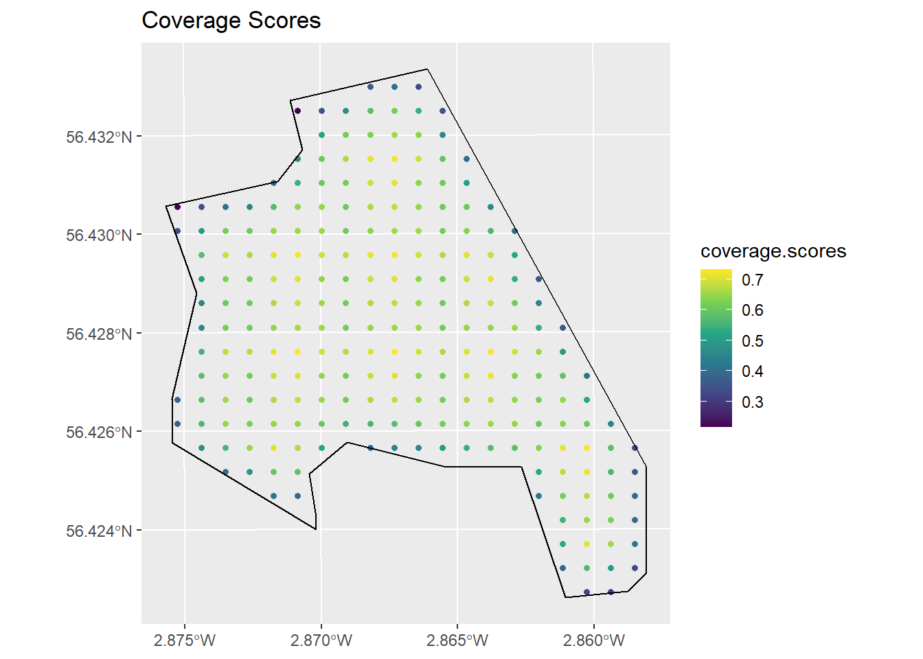
Does it appear that you that there is even coverage within strata?
The main strata looks to have fairly uniform coverage. The values appear to have such small levels of variability that the variability that is seen will be down to stochasticity as it is seen across the entire strata. The Morton Lochs strata we can see has areas of lower coverage around the edge of the study region. This grid is a bit too coarse to allow us to properly judge how much of an issue edge effects will be in this strata. It may be wise to re-run the coverage simulation with a finer coverage grid and more repetitions too. Edge effects could potentially be problematic in such small areas.